This article is about comparing different camera formats performance relative to each other within the context of image quality. Most of the article does not consider actual products on the market of their particular performance curves, but instead explains the principles on how different formats compare to each other which can be very useful for many purposes. The content is geared towards digital camera systems, but the relevant parts are valid for film as well as they’re universal.
I’ve divided the this post into three parts – the first one concerns about the formats and lenses, while the second considers certain performance metrics of image sensors which influence format comparisons. The third part shows an example with real digital cameras.
Formats and lenses
 The field of view (i.e. angle of view) depends on two parameters: focal length of a lens (ƒ) and size of the format. If one of the parameters change, the field of view will also change. To have a fixed field of view both parameters need to be change by the same factor. For example to have the same field of view a format with half the linear dimensions will have to use a lens with half the focal length.
F-number tells diameter of aperture at certain focal length: 
As exposure tells how much light is collected per unit area, if the total area – the format – is changed, the total amount of light captured changes as well. If we want to collect the same amount of light with different formats, we have to use different exposure settings. We can either adjust the shutter speed, or the scene luminance, or the aperture number. If we change the aperture number, we also change the depth of field (DoF) – interestingly if we adjust the aperture number so that the depth of field becomes the same, both aperture diameter and amount of light collected is equalled as well (*). The relevant formulas will follow in this article.
Relevant formulas for depth of field according to Wolfram Alpha are:


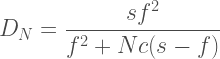
DoF = depth of field
ƒ = focal length
N = f-number
s = focus distance
c = circle of confusion
DF = far limit of depth of field
DN = near limit of depth of field
Thus to draw the same image with different formats both the focal length and the aperture number have to be adjusted by the relevant ratio of the formats’ diagonal sizes.
It is good to know that the above formula may not give valid results if the focus distance is small (e.g. macro photography or close-ups). For such we can use this formula instead:

Where m is magnification. It’s good to remember that for the same framing different formats will have different magnification (the relation is the inverse of the crop factor, e.g. to match the framing of APS-C with crop of 1,5 and magnification of 1, a full frame camera would use magnification of 1,5).
It is also good to consider the “working f-number” or “effective f-number” which is relevant at close focus distances. This is calculated simply using this formula: N(1+m), where N is the f-number and m is magnification.
Also one should pay attention to the magnification – it is simpy f/(s-f) where s is subject distance and f is focal length.
Also, at macro distances angle of view is not the same as it is at infinity.
So this can get complex even when one simplifies things which has been the case above. I image this is worth anohter article!
Noise vis-à-vis format
Light is by it’s very nature noisy as light particles, photons, live and die according to the rules set by Schrödinger’s cat – quantum mechanics. We can largely forget this now and just remember that when light is detected, it’s particles will follow Poisson distribution – this is why there is photon shot noise which is by far the dominant source of noise in output images. Noise is usually considered to be equal to the standard deviation of the signal. For light this is trivial to calculate since in Poisson distribution the standard deviation is equal to the square root of the mean!
The image sensor generated noises are not considered at all outside of the real world calculation at the end of the article as in the context of comparin format they are usually not relevant for modern image sensors in typical use.
Because of this it is also easy to calculate how much changing the size of the format changes the amount of signal, noise and their ratio (SNR). The answer is simple: if you double the area of the format, you improve the SNR by factor of square root of two (√2 ≈ 1,414). If you double the diagonal of the format (“crop factor”), you quadruple the area of the format and double the SNR (with the caveat of aspect ratio differences). It is indeed signal to noise ratio which is of interest, not noise by itself.
The reason for above is because signal noise add up differently. Adding signals is as simple as S = S1 + S2, but uncorrelated noises add up in quadrature: N2 = N12 + N22 ⇒ N = √(N12 + N22).
Thus if we multiply the format area by a, then signal SB = aSS. But noise NB = √(aNS2) = √a√Ns2 = Ns√a. Thus SNR increases at the rate of √a. If instead we consider format diagonal, then for images of same aspect ratio SNR increases at by the very amount were increase the diagonal – for example if we compare APS-C image of “crop factor” of 1,5 to a full frame image, the latter will have SNR that is 1,5 times larger!
Collecting the same light
If we have a fixed angle of view, the cone of light which hits the lens is the same. How much of that light goes through the lens is defined by the diameter of the aperture of the lens. The wider the cone of light is, the more light hits the lens and the smaller the aperture diameter can be for the same light to go through. This is why a long tele lens has a very large aperture (and front element) while a wide angle lens at the same maximum f-number will have just a tiny aperture (and can have a tiny front element too). This is good to know, since when calculations involve the aperture diameter, the angle of view should be identical as well, thus “crop factor” should be applied to the focal length – that it is precicely the crop factor can be easily seen from the basic formula for angle of view:
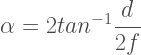
α = angle of view
d = diagonal of the image sensor
f = focal lengh
To get the same noise from different formats one needs to get the same light through the lens to the sensor. Lets consider angle of view, scene luminance and exposure time to be fixed – now the only parameter which dictates how much light hits the image sensor is size of the aperure. If we fix that too, then the same light will go through. As aperture diameter is focal length divided by the f-number, adjusting focal length by the “crop factor” requires adjusting aperture number by the same factor in order to maintain the same light collection. For example if you were to divide focal length by two, you’d have to divide the aperture number by two to collect the same amount of light.
Collecting the same amount of light means that the signal to noise ratio (“noise”) is the same. Thus to get the same noise performance with fixed scene luminance and exposure time the f-number will have to be adjusted by the crop factor – bigger number for bigger format, smaller number for smaller format.
Out of focus blur
In the context of comparing formats it’s best to consider this nice formula:

c = circle of confusion
A = diameter of entrance pupil
m = magnification
S1 = focus distance (from entrance pupil)
S2 = out of focus distance (from entrance pupil)
The sensor format size itself is irrelevant as we can directly consider the output image (“print”) magnification and circle of confusion instead of the respective parameters of the image sensors. Thus when comparing different sensor formats the out of focus blur is the same if the diameter of the entrance pupil is the same.
Thus “crop factor” adjustment applies to the f-number regarding out of focus blur as f-number is simply the ratio of focal length and entrance pupil diameter.
Diffraction versus format
For diffraction influence on the output image with different formats we can consider the following simple formula:

r = Radius of the Airy disk
λ = wavelength of light
N = aperture number (the “f-number”)
It is trivial to see that that if we double the f-number, we double the diameter of the airy disk. Because the image is different size for different formats, the enlargement for the output image will also be different, thus the effect of the radius of the Airy disk (and diffraction) will be different.
It is easy to understand that if the enlargement from one image to a fixed sized output image (“print”) is twice that from what it’s from another image, the respective Airy disk will have to be half the diameter to maintain the same diffraction effect. For example f/4 on one system has the same diffraction effect f/2 has on a system which has image sensor half the diagonal size.
Thus “crop factor” adjustment applies to the f-number regarding the effect of diffraction.
Consequences of format differences
If we consider systems which have common signal collection efficiency limitations we can consider four different shooting conditions (assuming fixed scene luminance):
- If exposure time is fixed, but depth of field is not, then a larger sensor can have SNR advantage, but to achieve that the depth of field will have to be more narrow.
- If depth of field is fixed, but exposure time is not, then the larger sensor can have SNR advantage, but to achieve that it needs to use a slower shutter speed.
- If both exposure time and depth of field are fixed, then the SNR is the same, regardless of format.
- If both exposure time and depth of field can float freely, the larger sensor will have SNR advantage.
In essence one can get better signal to noise ratio if one is willing to trade either space or time to get it, thus to get it either a longer exposure or more shallow depth of field is required. The limits for SNR correlate with the size of the format which is used.
The above provides a good framework for cross format comparisons and works splendidly when the image capturing devices are clones of each other, just perfectly scaled to different formats. This is of course a rather idealized situation when it comes to image sensors, though works well with film.
What kind of deviations from the above are to be expected when using actual real world digital cameras is a topic which is considered later in this article.
Optical phenomena vis-à-vis format
While this article is mostly about image quality from the signal to noise ratio’s point of view for the sake of completeness it’s a good idea to touch some other points which are relevant to image quality.
By definition different formats have different physical image size – to get to desired physical output size the image size has to be adjusted, typically enlarged significantly from maybe a couple of centimetres diagonal to ten or more times that. The more the image is enlarged the more all the imperfections as drawn by then lens will manifest themselves. Thus to get the same optical image quality the smaller the format, the better the optics will have to be.
Diffraction is an image blurring phenomenon which has the same effect to the output image on all formats if the depth of field is the same. The lens aperture ranges of different formats tend to offer the systems somewhat differing ranges of depth of field options with the smaller ones having apertures allowing for very deep depth of field, but which is severely resolution limited by diffraction, while the larger formats tend to have possibilities for more narrow depth of field with lower diffraction, thus higher potential for resolution. In practise the wide depth of field advantage of smaller formats is largely, if not entirely, removed because of the amount of diffraction, and the extra resolution potential of larger formats at narrow depths of field is not realized because of coarse image sampling (and possibly aberrations of the lenses).
Depth of focus is to the image what depth of field is to the subject. When the magnification of the subject is small, we can simplify the relevant formula to just t ≈ 2Nc, where t is the depth of focus, N is the aperture number, and c is the circle of confusion. Circle of confusion (CoC) scales directly with the linear size of the format – the bigger the format, the bigger the CoC. For the same depth of field, the aperture numbers will be different for different formats – also scaled according to relevant format sizes. What this means is that the smaller format will have much finer depth of focus than the larger format if the depth of field is the same. This means that there is much less tolerance for lens manufacturing errors and that to achieve the same focusing accuracy much finer focusing has to be performed. If we consider crop-factors, then the depth of focus difference for the same depth of field scales by factor of r2, where r is the relevant crop factor.
Influence of image sensor properties
I will consider the effects of quantum efficiency, full well capacity and read noise of different image sensors in this part of the article as they influence the practical camera comparisons directly. I will not consider for example the properties of the colour filter array even though it also has an effect on the noise and quality of the output image to keep things as simple as possible and will thus only consider the most important aspects.
Quantum efficiency (QE) tells how large number of the photons that reach the image sensor are detected and recorded by the sensor. There are different variation of the concept, but this definition fine for us. Different image sensors have different QE, though the difference is usually very small among sensors of the same generation. At the time of writing of this article a typical image sensor has approximately 50% QE.
Full well capacity (FWC) tells us how many photons a pixel can collect and record (in electrons) before the pixel saturates (i.e. reaches the maximum signal level). FWC can be just a few thousand for small pixels, but over 100.000 for large ones (for consumer cameras) at the time of writing.
Read noise (RN) is the amount of noise the sensor itself injects into the signal of a pixel. While this is not a monolithic singular noise, but a combination of multiple noise sources, for the purposes of this article there is no need to consider the separate components. We can also consider read noises of the pixels the be uncorrelated as that is largely the case for the relevant components. The transistor sharing schemes can complicate things if we want very high degree of accuracy for considerations though and that’s beyond this article. As of today typical RN is about 3 or 4 electrons with some notable exceptions.
Shot noise (SN) is the noise of the light itself. It’s easy to think that light is not noisy as we don’t see such phenomenon with our eyes, but the physics of light is in reality quite different and noisy. Fortunately the noisy nature of light follow the Poisson distribution, thus the noise, or the standard deviation is simply the square root of the signal. Shot noise is also uncorrelated.
If we were to compare image sensors with the same number of pixels, things are easy and we can consider the above values themselves. But if not, we need to make adjustments to FWC and both kinds of noises. Simply FWC (and signal) goes up by the number of pixels, but noises by the square root of the number of pixels – the latter is because noises add up in quadrature, i.e. N2 = N12 + N22.
An example
For the comparisons I use the sensorgen.info database which is derived from the data of DxOMark. The accuracy of the derived numbers is not always too good, so they should not be treated as divine truth, but as approximations.
Sony A7 vs. Olympus OM-D-E-M1
The Sony A7 has an image sensor which has 24240576 pixels, while the Olympus as 16110080 pixels. The Sony has QE of just 42%, the Olympus 48%. The Olympus pixels have a full well capacity (at the base ISO) of 16234 electrons, Sony’s bigger pixels 51688 electrons. The read noise of Olympus is 2,9 electrons, Sony’s 4,9 electrons, again at base ISO. The signal is anything between zero and FWC.
Because the pixel counts differ, we need to do normalize some of the numbers. The sum of the full well capacities are the pixel counts multiplied by the FWC and the sum of signals is signals multiplied by number of pixels as well. The sum of read noises are the read noises multiplied by the square root of the number of pixels. The sum of shot noises is the square root of the signal multiplied by the square root of the number of pixels.
Thus for saturation (signal = 100% FWC) the Sony has 125,29469×10⁹ electrons. The sum of shot noises for whole sensor at saturation is 1119351,1 electrons, the sum of read noises 10898,57 electrons – the sum of these sums is added in quadrature, thus it’s 1119404,2 electrons: at saturation the read noise is quite irrelevant.
For Olympus the sum of saturations is 26,153103872×10⁹ electrons, and the relevant noise sums are: shot 511401,05 electrons, read 6835,1468 electrons and total 511446,73 electrons.
If you’re interested in for example middle grey performance, you’d set the signal of a pixel to be 18% (or whatever is considered to be middle grey) of FWC and calculate shot noises from that. Or if you want to go down 6 stops from saturation, you’d use signal of 1,5625% of FWC and shot noise based on that signal.
Let’s consider the two possibilities:
- If exposure is not limited, at maximum signal level the A7 has about 2,18 times better SNR.
- If exposure parameters as fixed (i.e. same DoF and exposure time and scene luminance), and exposure is limited below Olympus saturation level, then the Olympus will collect 48%/42%=1,14 times more light, and at the saturation point of Olympus it would have about 7% higher SNR than the Sony!
If we consider a situation eight stops below saturation (0,4% of saturation), deep shadows:
- Unlimited exposure: A7 will now have 2,21 times better SNR.
- Limited exposure to 0,4% of Olympus saturation (e.g. we want certain DoF and shutter speed on fixed scene luminance): Olympus now has 11% better SNR!
Conclusion
The SNR between different cameras of formats under different shooting situations follows closely the theoretical performance ratios of the situations presented earlier where the maximum SNR ratio is the square root of the ratio of sensor surfaces (i.e. approximately the ‘crop factor’) and the minimum ratio is one, i.e. no difference. If the camera sensors are of significantly different capabilities the relevant SNR ratios may change by significant margins, but on the other hand image sensors of roughly the same generation will not demand much consideration regarding SNR adjustments.
Essentially for same generation of sensors the following is true with for most part only minor adjustments, and to reasonable accuracy with no adjustments at all:
- If exposure time, depth of field and scene luminance are fixed and no overexposure happens, then the SNR is the same, regardless of format.
- Otherwise the larger sensor will have SNR advantage equal to the relevant crop factor if the sensor’s superior potential is used fully.
(*) There is a small caveat – if the focus distance is very small compared to the focal length (e.g. macro regime), the equality vis-a-vis depth of field collapses and the larger image sensors will have larger depth of field at “equivalent settings”.
